
The Curious Case of 15 Lost Tosses: Modeling the Odds
How rare was India’s 15-toss losing streak?

The Data Signal is a free newsletter for data analytics & product enthusiasts. Hit the nifty button below to subscribe and never miss a post!
India played New Zealand in the Champions Trophy final on 9th March 2025. While I don’t follow cricket regularly, I found something interesting: India’s captain, Rohit Sharma, lost his 12th toss in a row, and for India, it was the 15th consecutive loss! Rohit Sharma joined Brian Lara of the West Indies in this dubious record.
A few news portals reported that the probability of losing 15 tosses in a row is 0.0000305.
This is where my interest peaked. I started wondering how they were calculating this probability. I suspected they might be calculating the probability of getting consecutive heads/tails—not necessarily losing the toss. So, I asked four of my friends—Claude, Gemini, DeepSeek, and ChatGPT—this question: “Calculate the probability of losing 15 tosses in a row.”
All of them gave me the same answer: 0.0000305, which was also reported by these news websites.
So, on a lazy Sunday evening, I decided to model it myself.
In this blog post, I will take you—the reader—through my approach, especially how I thought about this problem. This may not be the only way to solve it, but it provides a useful framework for thinking about probability in such cases. Before we begin, let’s acknowledge one thing: this is a very rare event. We are simply trying to gauge the degree of rarity.
I am sharing snippets of my R code with my commentary. The GitHub link is here. (It is a bit messy as it was mostly exploratory work)
First, we will randomly generate toss outcomes—H or T—with equal probabilities. Then, we will randomly generate the call—H or T—with equal probabilities.
library(ggplot2)
library(tidyverse)

# Generate two vectors - one for the toss outcome, one for the actual call

num_samples <- 15
toss_outcome <- sample(c("H", "T"), num_samples, replace = TRUE, prob = c(0.5, 0.5))
actual_call <- sample(c("H", "T"), num_samples, replace = TRUE, prob = c(0.5, 0.5))
Next, we decide the winner. If the toss outcome and call are the same, then the winner is the “Caller”; otherwise, it’s the “Watcher.”
#Create a dataframe

cbind(toss_outcome, actual_call) %>%
  as.data.frame()-> toss_df

#Add Caller or Watcher

toss_df %>%
  mutate(winner = ifelse(toss_outcome==actual_call, "Caller", "Watcher"))-> toss_df
From here, we can calculate the percentage of instances where the Watcher wins and the percentage where the Caller wins. Let’s wrap this in a function that takes the number of coin tosses as input and returns the winning percentage for the Caller.
TossSimulation <- function(num_samples = 15) {
  toss_outcome <- sample(c("H", "T"), num_samples, replace = TRUE, prob = c(0.5, 0.5))
  actual_call <- sample(c("H", "T"), num_samples, replace = TRUE, prob = c(0.5, 0.5))
  toss_df <- cbind(toss_outcome, actual_call) %>%
    as.data.frame() %>%
    mutate(winner = ifelse(toss_outcome == actual_call, "Caller", "Watcher"))

  caller_perc <- toss_df %>%
    count(winner) %>%
    mutate(perc = 100 * (n) / sum(n)) %>%
    filter(winner == 'Caller') %>%
    pull(perc)

  return(caller_perc)
}
To check our intuition, we first simulate a large number of tosses. If we toss a coin many times, the probability of either side winning should approach ~50%.
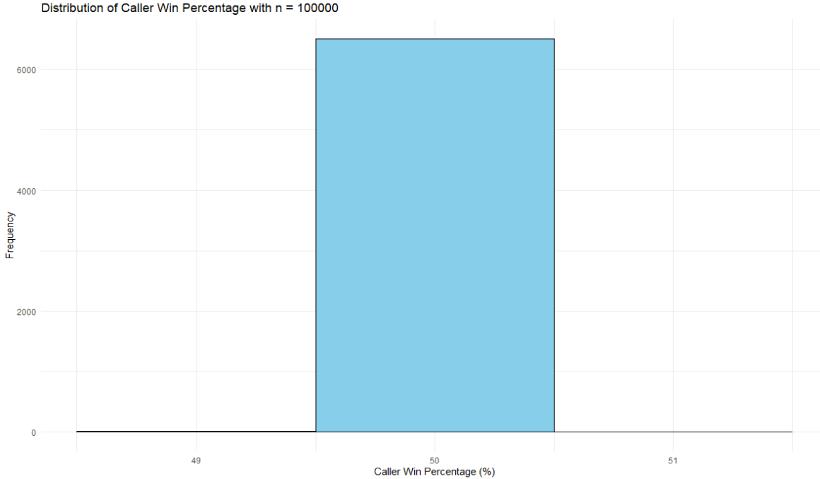
Running this function for a large number of trials (started with 10,000 but stopped around 6,500) confirmed this. The values were centered around 50%, with the lowest and highest being 49% and 51%, respectively.
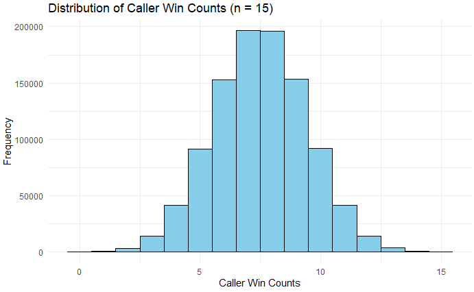
Now, let’s take this to the big game—15 tosses, repeated 1 million times. And instead of percentage, let’s take the count.
#Minor improvement added to calculate the cases when the Caller doesn't win any tosses

TossSimulation <- function(num_samples = 15) {
  toss_outcome <- sample(c("H", "T"), num_samples, replace = TRUE, prob = c(0.5, 0.5))
  actual_call <- sample(c("H", "T"), num_samples, replace = TRUE, prob = c(0.5, 0.5))
  toss_df <- cbind(toss_outcome, actual_call) %>%
    as.data.frame() %>%
    mutate(winner = ifelse(toss_outcome == actual_call, "Caller", "Watcher"))

  caller_count <- toss_df %>%
    count(winner) %>%
    filter(winner == 'Caller')

  if (nrow(caller_count) == 0) {
    return(0)
  } else {
    return(caller_count$n)
  }
}
results_vector_15 <- c()
for (i in 1:1000000) {
  results_vector_15[i] <- TossSimulation(num_samples = 15)
}
results_df_15 <- data.frame(count_wins = results_vector_15)

#Plot the distribution

ggplot(results_df_15, aes(x = count_wins)) +
  geom_histogram(binwidth = 1, fill = "skyblue", color = "black") +
  labs(title = "Distribution of Caller Win Counts (n = 15)",
       x = "Caller Win Counts",
       y = "Frequency") +
  theme_minimal()
The distribution looks much more ‘normal.’ So, what is the probability of someone winning (or losing) all 15 tosses in a row?
100*(results_df_15 %>%
  filter(count_wins==0 | count_wins==15) %>%
  nrow())/(nrow(results_df_15))

#output: 0.0075
Out of those 1 million trials, only 75 times did someone (including both Caller and Watcher) win or lose all 15 coin tosses. This translates to a probability of ~0.000075, or 1 in 13,333. This number is slightly different from the 0.0000305 quoted earlier, but it still confirms the rarity of the event.
How does this number change when we experiment with 12 consecutive toss losses? (Remember, this has already happened twice.)
The probability for 12 consecutive losses comes out to ~0.000258, which is 1 in 3,876.
Next, let’s examine how many sequences of 15 matches India has played since the beginning. India has played a total of 1,066 ODI matches. Here’s a simple way to understand how to count sequences of m elements within a list of n elements. Suppose we have five matches and need to count sequences of three consecutive matches. The number of sequences is three because we can start at any of the first three positions (the last two positions don’t allow for a full sequence of three).
Applying this to our case: the number of possible 15-match sequences is (1,066 - 15 + 1) = 1,057. This means we had 1,057 opportunities for a 15-match losing streak to occur. If the base probability was 1 in 13,333, then achieving this streak in 1,057 tries is still quite rare but not impossible.
This was a simple mental exercise to derive the probabilities. The analysis can be refined further using a Bayesian approach. For example, we assumed the toss call is 50-50. But what if Rohit and Lara prefer calling H over T, or vice versa? How would that affect the probability?
Is my math mathing for you? How would you think about this problem? How would you solve it?
If you found this breakdown interesting, share it with a friend who loves cricket, math, or a good statistical oddity!